Creating a Loadings Color Matrix Plot

Overview

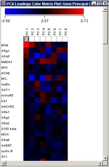
The Loadings Color Matrix Plot is one of three closely related plots (Loadings Line Plot, Loadings Scatter Plot, and Loadings Color Matrix Plot) that displays the individual elements the PCs. (Since a PC is a vector, it has constituent elements which are called the loadings. By mathematical definition of PC adopted by GeneLinker™, the Euclidean norm, i.e., vector length, of each PC is 1.) The loadings of a given PC represent the relative extent to which the original 'variables' (Genes or Samples, depending on the Orientation selected for the PCA) influence the PC. The Loadings Color Matrix Plot displays these loadings as a tiled grid of colored rectangles such as those typically used to view tables and clustering results.

The PCs are in the columns and the 'variables' are in the rows (e.g., Genes if PCA by Genes). The legend displays a color gradient, and the scale of values from the minimum to maximum coefficient value. Often there are so many variables in gene expression data that this type of visualization makes it easier to gain an overview and to interpret than the Loadings Line Plot and Loadings Scatter Plot.

The loadings (color-coded rectangular tiles) can be interpreted as the derived relative weightings of the original 'variables' in the derived linear combination that constitutes each PC. Thus, the color-coded tiles express the relative weights of association between the original 'variables' and the computed PCs.

The default sort for the Loadings Color Matrix plot is in absolute descending order of the first PC.

Actions

1. Click a PCA Experiment in the Experiments navigator. The item is highlighted.

2. Click the Loadings Color Matrix Plot toolbar icon , or select Loadings Color Matrix Plot from the PCA menu, or right-click the item and select Loadings Color Matrix Plot from the shortcut menu. The Loadings Color Matrix Plot is displayed.

Sorting by Principal Component

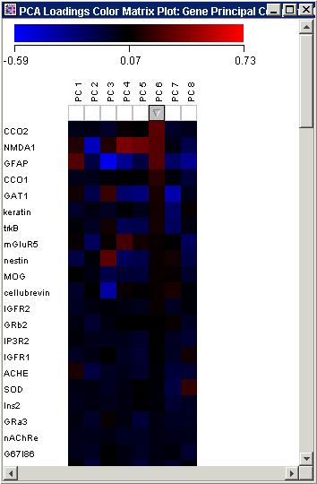
At the top of the plot, under each PC label is a button. Only one of these buttons is active at a time. It indicates the current plot sort and by which PC.

The rows of the plot can be sorted by a single PC in:

Absolute descending order (highest to lowest value regardless of sign).
Descending order (highest to lowest value).
Ascending order (lowest to highest value).

The default sort for the Loadings Color Matrix plot is in absolute descending order of the first PC.

To sort by a PC, click on the button under the PC label. This button operates in a cyclic fashion. The cycle is as follows:

1. Click once, the sort is in absolute descending order.

2. Click the same button again, the sort is in descending order.

3. Click the same button again, the sort is in ascending order.

Click the same button again and the cycle begins again (absolute descending order).

Each time a sort button is clicked, the plot is updated to reflect the new sort status. In the example below, the samples are sorted in descending order by the 6th PC.

Launching a Loadings Line Plot

1. Select one or more PCs by clicking on the PC label. Press and hold the <Ctrl> key to select multiple PCs. To select a series of PCs, press and hold the <Shift> key and click on the first and last PC labels in the series.

2. Select Loadings Line Plot from the PCA menu, or right-click on the color grid and select Loadings Line Plot from the shortcut menu.

Launching a Loadings Scatter Plot

1. Press and hold the <Ctrl> key and click on two PC labels.

2. Select Loadings Scatter Plot from the PCA menu, or right-click on the color grid and select Loadings Scatter Plot from the shortcut menu.

Other Plot Operations

Displaying Expression Values

Changing the Gradient Color and Scale

Resizing Cells in a Color Grid

Exporting a PNG Image