Platinum

Tutorial 6: Step 10 Display a Confusion Matrix

 View the Classify Results

1. If the newly created Predictions (or whatever name you gave the new classification in the previous step) item in the Experiments navigator is not already highlighted, click it.

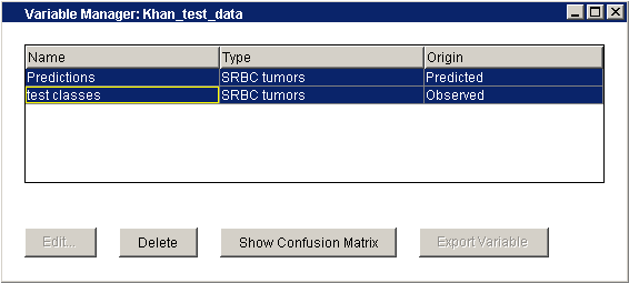
2. Select Variable Manager from the Tools menu. The Variables dialog is displayed.

You see a list of the variables GeneLinker™ currently has associated with the Khan_test_data dataset family. Each variable has a name, a type, and whether it was imported (Observed) or generated by a classifier (Predicted).

3. Click on test classes. It is highlighted.

4. Hold down the <Ctrl> key and click on the Predictions item. Both variables are highlighted.

5. Click Show Confusion Matrix at the bottom of the dialog. The Confusion Matrix plot is displayed.

Description of the Confusion Matrix

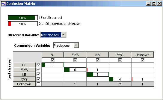
The confusion matrix is an array which summarizes the comparison between two variables relating to a dataset. Typically the variables are an observation and a prediction. Each row in the confusion matrix represents an observed class, each column represents a predicted class, and each cell counts the number of samples in the intersection of those two classes. Entries on the diagonal of the matrix (in dark green) count the correct calls or predictions. Entries off the diagonal (in red, if there are any) count the misclassifications.

At the top of the confusion matrix display are two bars representing the overall accuracy of the prediction and the error rate.

Observations labelled 'Unknown' are not included in calculating the accuracy of the learner, since they are taken to represent cases where the scientist really does not know the class of the sample. Therefore any prediction made by GeneLinker™ in these cases can neither be counted as correct or incorrect.

In contrast, a prediction of 'Unknown' from GeneLinker™ means that the program could not confidently assign a class to the sample. Such a prediction is counted as an error if there is an observed class available for the sample (that is, a class other than 'Unknown').

This behaviour of the confusion matrix summary can be modified by checking or un-checking the box at the left of each row and the head of each column. You can also use the checkboxes, for example, to restrict the accuracy summary to consider only two classes of a multi-class problem.

Discussion of the Example Data

Five samples in this test data do not belong to any of the four training classes: TEST-3, TEST-5 and TEST-11 are other cancers, and TEST-9 and TEST-13 are normal muscle tissue. They are labelled 'Unknown' in this tutorial and are represented by the last row in the confusion matrix above. Four of these five non-SRBCT samples are predicted to belong to one or the other of the training classes, which illustrates an important point: the classifier cannot be relied upon to detect classes which lie outside the domain of the training data. It tries, but it does not always succeed.

This is an important point about machine learning, and worth reinforcing with an imaginary example from human learning. Suppose a young child had seen lots of dogs, but never seen a wolf – not even a picture. When first presented with a picture of a wolf, the child will very likely proclaim 'Dog!' The child would probably do the same with a picture of a fox. Machine learners are no smarter, and in fact tend to be less able to distinguish outlying cases. When training a machine learner, it is important that the samples chosen for training represent all the classes that the learner will eventually be expected to distinguish.